SVM’s on Spam Filtering
Using SVM’s with polynomial kernels to detect spam email
Consider the binary classification that consists of predicting if the e-mail message if a spam using the 57 features. Use SVMs combined with polynomial kernels to tackle this binary classification problem. To do that, randomly split the training data into ten equal-sized disjoint sets. For each value of the polynomial degree, d = 1, 2, 3, 4, plot the average cross-validation error plus or minus one standard deviation as a function of C (let other parameters of polynomial kernels in libsvm be equal to their default values), varying C in powers of 2, starting from a small value C = 2−k to C = 2k, for some value of k. k should be chosen so that you see a significant variation in training error, starting from a very high training error to a low training error. Expect longer training times with libsvm as the value of C increases.
Lets start with preprocessing the data.
- Read the data
- Split the data into training and test test
- Transfrom data to work with lib-svm
- Normalize data and save the transformation with
-s myrangeflag. - Do the same for test set, using the scale factors used for training-set normalization using
-r myrangeflag
import os

f=open("sb.txt",'r') //data

x=[]
y=[]
for l in f:
    m_i=l.strip().split(',')
    y.append(int(m_i.pop()))
    x.append(map(float,m_i))
f.close
xtrain=x[:3450]
ytrain=y[:3450]
xtest=x[3450:]
ytest=y[3450:]
f=open("data","w")
for i,y in enumerate(ytrain):
    a=[str(j+1)+':'+str(e) for j,e in enumerate(xtrain[i])]
    if y>0: f.write('+1 '+' '.join(a)+'\n')
    else: f.write('-1 '+' '.join(a)+'\n')
f.close()
f=open("data.t","w")
os.system(' ../svm-scale -s myrange data > datascaled')
for i,y in enumerate(ytest):
    a=[str(j+1)+':'+str(e) for j,e in enumerate(xtest[i])]
    if y>0: f.write('+1 '+' '.join(a)+'\n')
    else: f.write('-1 '+' '.join(a)+'\n')
f.close()
os.system('../svm-scale -r myrange data.t > datascaled.t')
0
Here 0 is received from os.function means successful termination. Lets train with 10-fold cross validation
from svmutil import *
import random as r
import numpy as np
from IPython.display import clear_output
K=10
k=10
drange=[1,2,3,4]
y, x = svm_read_problem('datascaled')
err=np.zeros((10,k*2+1,len(drange)))
totalmodelnum=K*(k*2+1)*len(drange)
counterr=0;
for i in range(K):
    starti=345*(i) #3450/10
    endi=345*(i+1)
    xtest=x[starti:endi]
    ytest=y[starti:endi]
    xtrain=x[:starti]+x[endi:]
    ytrain=y[:starti]+y[endi:]
    for d in drange:
        for c in range(-k,k+1):
            counterr+=1;
            m = svm_train(ytrain, xtrain, '-c '+str(2**c)+ ' -t 1 -q -d '+str(d))
            p_label, p_acc, p_val = svm_predict(ytest, xtest, m)
            err[i][c+k][d-1]=p_acc[0]
            clear_output(wait=True)
Accuracy = 94.7826% (327/345) (classification)
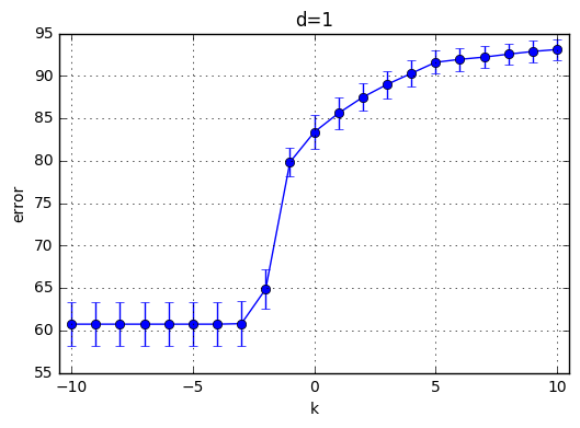
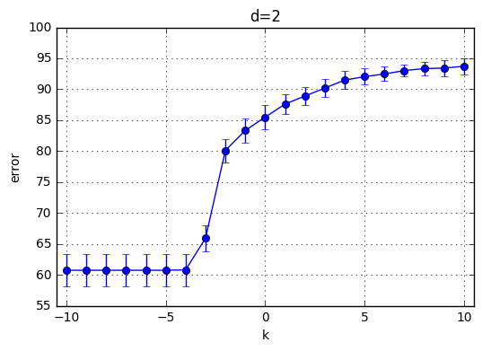
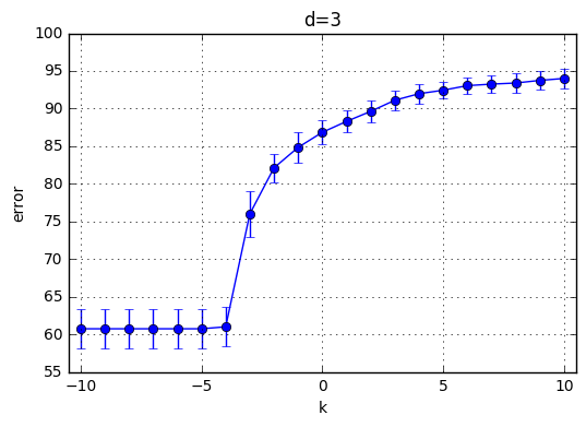
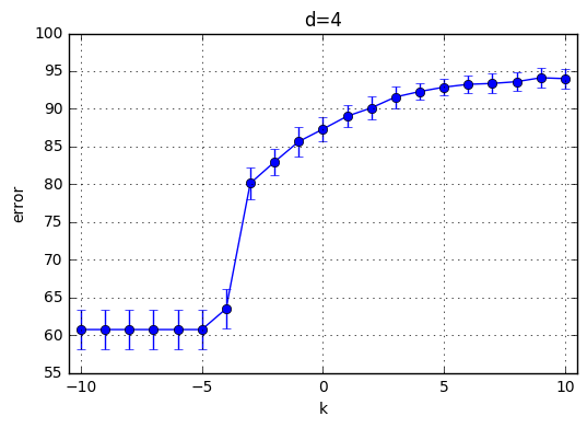
I’ve trained \(C(Error Term)*d(polynomial degree)*CrossValidation = 21*10*4=820\) model and the results are highlighted below. First observation is with the increasing degree of the polynomial kernel the model reaches its maximum performance earlier. In other words, for the small C values, the model performs poorly and around a specific C the mean accuracy starts increasing. This starting value of C is shifted towards left with increasing C. With increasing C the accuracy increases for each model and the variaton decreases.
Best performance observed generated by the choice of k=9 and C = 29. Therefore I’ve chosen C = 512 for the next part.
import numpy as np
import matplotlib.pyplot as plt

x = np.array(range(-k,k+1))
for d in drange:
    y = np.mean(err[:,:,d-1],0) # Effectively y = x**2
    e = np.std(err[:,:,d-1],0)
    plt.subplot(111)
    plt.errorbar(x, y, yerr=e, marker='o')
    plt.ylabel('error')
    plt.xlabel('k')
    plt.title('d='+str(d))
    plt.grid(True)
    plt.xlim(-k-0.5, k+0.5)
    plt.show()
totald=31
drange2=range(1,totald)
y, x = svm_read_problem('datascaled')
err2=np.zeros((K,totald-1))
totalSVs=np.zeros((K,totald-1))
onplaneSVs=np.zeros((K,totald-1))
models=[]

for i in range(K):
    models.append([])
    starti=345*(i) #3450/10
    endi=345*(i+1)
    xtest=x[starti:endi]
    ytest=y[starti:endi]
    xtrain=x[:starti]+x[endi:]
    ytrain=y[:starti]+y[endi:]
    for d in drange2:
        m = svm_train(ytrain, xtrain, '-c 512 -t 1 -q -d '+str(d))
        models[i].append(m)
        p_label, p_acc, p_val = svm_predict(ytest, xtest, m)
        err2[i][d-1]=p_acc[0]
        #Now find the total number svs
        totalSVs[i][d-1]=m.get_nr_sv()
        #Now find SV's on hyperplane
        inds=m.get_sv_indices()
        coeffs=m.get_sv_coef()
        yt=[ytrain[bb-1] for bb in inds]
        c=0
        for kth in range(len(coeffs)):
            yiwxib=yt[kth]*coeffs[kth][0]
            if yiwxib!=512:
                c+=1
        onplaneSVs[i][d-1]=c
        print i+1,'th Fold: d=',d
        clear_output(wait=True)

yrealtest, xrealtest = svm_read_problem('datascaled.t')
err3=np.zeros((totald-1))
for d in drange2:
        m = svm_train(y, x, '-c 512 -t 1 -q -d '+str(d))
        p_label, p_acc, p_val = svm_predict(yrealtest, xrealtest, m)
        err3[d-1]=p_acc[0]
        clear_output(wait=True)
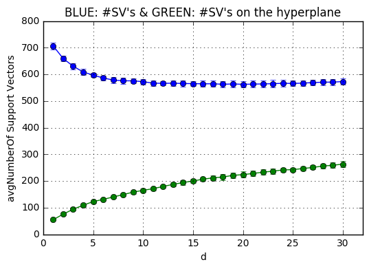
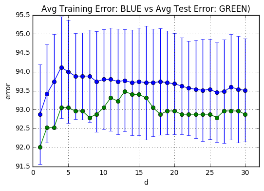
The next code snippets plots the average number of support vectors averaged over the k-fold trained models(BLUE) and the amount of which lie on the hyperplane(GREEN) for each $d \in [1,31]$. The support vectors which are on the plane are calculated through non-zero coefficients. When a support vector is not on the hyper plane, then its coefficient $\alpha_i$ becomes 512(C)
import numpy as np
import matplotlib.pyplot as plt
x = np.array(drange2)
y1 = np.mean(err2[:,:],0) # Effectively y = x**2
e1 = np.std(err2[:,:],0)
y2 = err3 # Effectively y = x**2
plt.subplot(111)
plt.errorbar(x, y1, yerr=e1, marker='o')
plt.errorbar(x, y2, marker='o')
plt.ylabel('error')
plt.xlabel('d')
plt.title('Avg Training Error: BLUE vs Avg Test Error: GREEN)')
plt.grid(True)
plt.xlim(0, totald+1)
plt.show()
meanSVs = np.mean(totalSVs[:,:],0) # Effectively y = x**2
stdSVs = np.std(totalSVs[:,:],0)

meanSVsOP = np.mean(onplaneSVs[:,:],0) # Effectively y = x**2
stdSVsOP = np.std(onplaneSVs[:,:],0)

plt.subplot(111)
plt.errorbar(x, meanSVs,yerr=stdSVs,marker='o')
plt.errorbar(x, meanSVsOP,yerr=stdSVsOP,marker='o')
plt.ylabel('avgNumberOf Support Vectors')
plt.xlabel('d')
plt.title('BLUE: #SV\'s & GREEN: #SV\'s on the hyperplane' )
plt.grid(True)
plt.xlim(0, totald+1)
plt.show()