
A very short review of Compressing Neural Networks
As my final project for the Computer Vision class tought by Rob Fergus in Fall 2016, I got the project of implementing compression ideas of Song Han presented in paper Learning both Weights and Connections for Efficient Neural Networks. Here is a very short review of the paper and some more.
Weights and Connections for Efficient Neural Networks
Song Han starts the paper with a focus on energy consumption of neural networks and motivates the need of compressing neural networks by pointing out that a smaller network would fit in memory and therefore the energy consumption would be less. He first talks about the Related Work
Related Work
- He first points out several quantization and low-rank approximation methods and says that those methods are still valid and can be applied after network pruning.[11-12-13-14]
- Then he mentions two methods utilizing global average pooling instead of the fully connected layer. I think this idea follows the fact that most parameters in popular models are due to the fully connected layers. [15-16]
- Then he mentions the early pruning ideas e.g. biased weight [17] decay and some others [18-19]
- Lastly the Hashed Nets are mentioned and an anticipation about pruning may help it presented[20]
Learning Connections in Addition to Weights
To prune the network importance of each weight is learned with a training method that is not mentioned. After this learning step, connections whose importance weights below a certion threshold are removed. Then the network is retrained and this part is crucial.
- Regularization: L1 and L2 regularizations are used during training and it is observed that even though L1(forces sparse weights) gives better after pruning accuracy, the accuracy after retraining observed to be better with L2
- Dropout Factor: Dropout should be adjusted during retraining due to the pruned connections with \(D_{new}=D_{old}\sqrt{\frac{C_{new}}{C_{old}}}\)
- Local Pruning and Parameter Co-adaptation: No reinitilization is made after pruning because it is obviously stupid to do. You can just train with smaller size if that was possible. ConvNet part and Fully Connected Layer’s are pruned separetely. It is mentioned that computation is less then original since partial retraining is made. I am not sure why this is not made layer by layer if vanishing gradients are the problem.
- Iterative Prunning: Prunning made through iterating and doing greedy search at each iteration. I am not sure which algorithm greedy search supposed to point here. It is a vague term. Doing one pass agressive prunning led bad accuracy.
My guesses about about iterative greedy search are:
- Choose threshold iteratively.
- ?
- Pruning Neurons Neurons are removed if there are either no incoming or no outgoing connections before retraining.
Experiments
Caffee is used and a mask is implemented over the weights such that it disregards the masked outparameters.
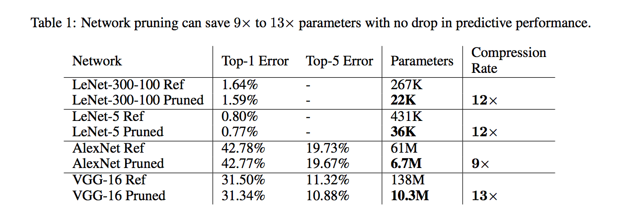
- Lenet5: After pruning retrained with LR/10 and a nice visualization is provided to show the outside weight are pruned(attention) [ ] Check: weights and importance weights give simalar plot like this.
- Alex-Net: 73h to train on NVDIA Titan X GPU. 173h to retrain with LR/100.
- VGG: Most of the reduction is at fully connected layer.
Discussion
There is still one point that is not clear to me how the pruning is made with L1 or L2. I need to think about this. But basically in this section it is shown that iterative prunning with L2-regularization gave best results. One need to prune different regions separetely. Because FC layers are more prunable.
- There is a free launch, which is prune %50 without retraining, same accuracy.
- Layers are pruned layer by layer. Sensitivity increases with deepness of the layer. It is not mentioned but the reason might be that the initial results effect more results and it may propogate and increase!
- Each layer’s sensitivity is used as threshold to prune each layer.
- Pruned layers are stored as a sparse matrix (a overhead of 15%, probably binary mask).
- Weight distribution of before/after pruning is given. Weights around 0 is disapeared.
Other Related Papers
Sparse Convolutional Neural Networks, Liu et. al.
I haven’t fully dived in to the decomposition part, but lets reflect on it.
- Uses matrix decomposition to get sparse parameters with an accuracy-sparsity tradeoff.
- After decomposition the model is retrained with regularization paramaters on the decomposed matrices.
- A sparse matrix multiplication algorithm is devised to utilize sparsity in the conv-layers.(256 bit AVX registers etc.)
- The algorithm is applied to the Imagenet CNN model in caffe.
- Decreased accuracy around 2%
Learning Structured Sparsity in Deep Neural Networks, Wei Wen et. al
- Structured Sparsity Learning(SSL) they name their algortithm.
- They use group lasso to obtain sparsity in different levels like row-column-filtersize-depthwise.
- Didn’t understand how they pick group lasso parameters(there are 4 of them I think)
- They provide really small speedups for Song Han’s prunning method. Even sometimes slow down
Optimal Brain Damage, LeCun et. al.
Yann Le Cun’s pruning paper emphasizing the importance of pruning as a regularizer and performance-optimizer. The idea of deleting parameters with small saliency is proposed. Magnitude of weights proposed as simple measure of saliency in the earlier literature and its similarity to the weight decay mentioned. This paper proposes a better more accurate measure of saliency.
- Saliency = change in the error function by deleting the parameter: HARD to COMPUTE
- Taylor Series Approximation: \(\delta E=\sum_{i}g_i\delta u_i + \frac{1}{2}\sum_{i}h_{ii}\delta u_i^2 + \frac{1}{2}\sum_{i\ne j}h_{ij}\delta u_i \delta u_j + O(||\delta U ||^3)\)
The first term is neglected, since it is assumed that the model is converged and gradients are near zero. The third term is neglected by assuming \(\delta E\)’s of each parameter is independent of others and therefore the overall \(\delta E\) is equal to the sum of individual \(\delta E\)’s. The last term is also neglected since the cost function is nearly quadratic. Then we left with:
\[\delta E=\frac{1}{2}\sum_{i}h_{ii}\delta u_i^2\]- Diagonal approximation of hessian matrix is calculated by (where \(V_k\) is set of connections sharing the same weight):
- The recipe of pruning connections according to the second order approximation given in the paper, where at each iteration some portion of the lowest saliency connections are pruned.
- A clear improvement over magnitude based prunning reported.
- A really interesting result is reported, too. MSE is increased aroun 50% percent after iterative pruning, however the test accuracy decreased, which is a clear indication showing the importance of loss function, i.e. MSE is not the right metric.
Pruning Convolutional Neural Networks for Resource Efficient Transfer Learning, Molchanove et. el.
This paper focuses on some transfer learning tasks where the models trained on Image-net transfered to solve smaller classification problems. One significant difference is instead of pruning weights whole neuron is pruned.
- The method is same:
- transfer&converge
- iterate with prune+retrain
- Stop when the goal is reached
- They used Spearman’s rank correlation to compare different saliency metrics with the optimal ‘oracle’ method(prune and measure \(\delta E\)), even though they pick only one neuron at each time.
- First order Taylor approximation gives best results compare to 1)sum of weights(of a neuron) 2)mean 3)std 4)mutual info, which is trivial and expected. Why should mean of weigths of a neuron be a metric for pruning…
- The first order approximation is basically the first term in the functions above
Comparing Biases for Minimal Network Construction with Back-Propagation, Hanson et. al.
It always feels good to read old papers. I visited this paper to learn more about Weight Decay and its connection to bias function(regularizer). They reported sparser connections are achieved as a result of applying exponential bias.
Expoloiting Linear Structure Within Convolutional Networks for Efficient Evaluation, Denton et. al.
This paper proposes around 2x speedup at convolutional layers by deriving low-rank approximations of the filters and 5-10x parameter reduction at fully connected layers. The motivation of the paper based on the findings of Denil et al. regarding the redundancies in network parameterts.
- First filters of first two convolutional layer is clustered into equally sized groups.
- For each group a low-rank approximation calculated by using SVD
Deep Comprression: Compressing Deep Neural Networks with Pruning, Trained Quantization and Huffman Coding
The main paper published at ICLR 2016 combining pruning idea with other methods like quantizing and huffman coding.
- The pruning part explained rather short and they emphasize that they laern the connections, with a regularizer.
- Quantization and weight sharing done first doing k-means clustering for each layer.
- They compared three intilization method for clustering and linear initiliaziation works best, since it keeps the high value weights.
- Shared weights tuned with backprop.
- It is shown that quatization works better with pruning.
- After all tuning is done, huffman encoding is made to comress the data offline.
- Up to 40x compression rate reached as a result.